Representation Learning: Inference for nothing and your accuracy for free

This evening, I’ll be talking about autoencoders. (Again.) I’ve been really liking unsupervised learning lately, apparently.

The motivation behind this demo is that:

1. We want as much labeled data as possible to make a useful predictive model.
2. Labeled data is expensive, but unlabeled data is cheap.
3. You can use your unlabeled data on your labeled data to get more bang for your buck!

I don’t really have a fun story to motivate or otherwise provide context for this today, unfortunately. As a poor substitute for that, I’ll share that I’ve really been liking the country music coming out of Texas in the past few years: Norther by Shane Smith & the Saints, Have A Nice Day by Treaty Oak Revival, and Sellout by Koe Wetzel. Those three albums are all kinda under the country rock umbrella; the former is a little bit more mature and contemplative and closer to country, and the latter two, closer to the rock side of things, are kinda rowdy and ignorant. Lynyrd Skynyrd is my favorite band of all time, and those three make me feel almost like I did when I first listened to Skynyrd (beyond Sweet Home Alabama, Free Bird, and Tuesday’s Gone, which were all in the “helping dad replace cylinder heads” soundtrack growing up). My aesthetic taste definitely doesn’t fit what you’d expect out of a recreational computer science enthusiast, but you should definitely check all those out.

You can find the code for all this on my GitHub: https://github.com/christianbolinas/autoencoder-demo.

The Experiment

The experiment itself was pretty simple. The basic premise was that we were going to:

• see if we could use the large amount of unlabeled data to learn information (that is, make new features, or make new “columns” out of the previous columns) about the underlying structure of the data, then
• use that information to transform the small amount of labeled data, using PCA or an autoencoder, and
• see if training a model on those new features of the labeled data increases accuracy relative to just training with the original labeled data.

If you missed the previous post, PCA, which stands for principal component analysis, is a linear technique to make new features (columns in your dataset) in a lower-dimension space (your new data has less columns per row) than the original one it was in. An autoencoder is a simple kind of neural network that does the same thing, but in a nonlinear way.

Actually, PCA is a 1-layer autoencoder with no activation function. Even if PCA was invented in 1901 and autoencoders became a thing some 80 years after that.

Because I’m too lazy to find and clean and preprocess more data, we were working with the MNIST dataset again, which is a dataset of pictures of handwritten digits. (We’re trying to predict the intended meaning of those handwritten digits). To simulate a small amount of labeled data (for the classifiers) and a large amount of unlabeled data (for PCA/the autoencoder), I split the working set into a small amount of labeled points and discarded the labels of the rest. I used a logistic regression as my classifier to keep things nice and simple.

1. First, to serve as a control, I fit a logistic regression to that subset of labeled data.
2. Next, I fit another logistic regression to the 64 principal components (as found with the unlabeled data) of that same subset of labeled data.
3. Last, I fit yet another logistic regression to the best 64-dimension latent representation (as found with the autoencoder, again as found with the unlabeled data) to that same subset of labeled data.

Results: PCA vs Autoencoders

Here’s what I found:

Preprocessing Technique	Logistic Regression Test Set Accuracy
None	88.7%
PCA, 64 components	90.3%
Autoencoder, 64 dimensions	93.8%

With the null hypothesis that an autoencoder wouldn’t increase model test set classification accuracy, we can confidently reject that H_0. You’re welcome to compute the z-scores ;)

I also fit a SVM with a RBF kernel to half the labeled data we originally had. That got 96.9% accuracy, which, again, results in a statistically significant increase in test set accuracy over the best logistic regression model, while training with half the data. The same SVM fit to the entire training set got 97.9% accuracy. Sickening.

Here’s a 2-D visualization of what a subset of the test set looks like. We want to see clear clusters of colors that you could draw boundaries between.

I know, I used logistic regression, not a SVM. So the metaphor isn’t accurate. Sue me.

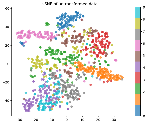
As you can see, with no transformation, you can’t really draw clear cluster boundaries. 4s and 9s are basically indistinguishable, and 0s are the only thing it does well-ish on. Here’s a visual of what PCA learned when squishing the data down:

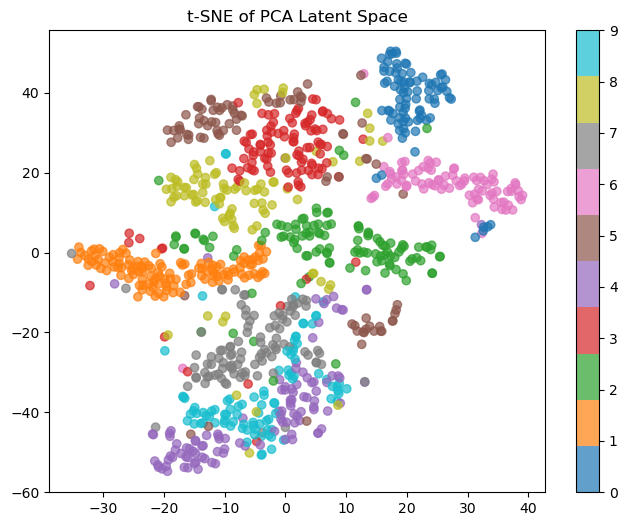
The clusters look like they’re slightly better quality, but 8s are still mixed in with the 4s and 9s (and also confused with 3s and 5s, which are themselves all over the place). Not great. Lastly, let’s see what the autoencoder learned:

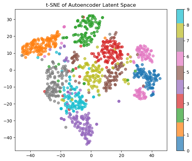
Much better. You can see actual clusters; the only issue is the 6s, which are split into two camps. If I had to guess, those would be those with a vertical versus sloped diagonals, but that’s an investigation for another day.

I hope this shows that unsupervised learning on cheap unlabeled data can help your inference on your labeled data. Thanks for reading!

Appendix: The Autoencoder

Here’s my model: I spent about five minutes coding it up for the previous post and copy-pasted it here, and didn’t do any kind of testing, cross-validation or otherwise, for a good architecture or hyperparameters. I used an Adam optimizer, a learning rate of 0.001, and trained on the unlabeled data for 10 epochs, which was a minute and 37 seconds on my laptop.

class Autoencoder_64(nn.Module):
    def __init__(self):
        super().__init__()
        self.encoder = nn.Sequential(
            nn.Linear(28 * 28, 512),
            nn.LeakyReLU(),
            nn.Linear(512, 256),
            nn.LeakyReLU(),
            nn.Linear(256, 128),
            nn.LeakyReLU(),
            nn.Linear(128, 64),
        )
        self.decoder = nn.Sequential(
            nn.Linear(64, 128),
            nn.LeakyReLU(),
            nn.Linear(128, 256),
            nn.LeakyReLU(),
            nn.Linear(256, 512),
            nn.LeakyReLU(),
            nn.Linear(512, 28 * 28),
            nn.Sigmoid(),
        )
    def forward(self, x):
        encoded = self.encoder(x)
        decoded =  self.decoder(encoded)
        return decoded
    def transform(self, x): # x is an ndarray
        self.eval()
        with torch.no_grad():
            out = self.encoder(torch.from_numpy(x).float()).numpy()
        return out