The Fast Fourier Transform and Kernels

Blah blah I didn’t use AI to write this, English or Python. I did use AI alongside youtube videos to learn about the FFT algorithm Pants-on-head AI use bad. Thoughtful AI use good. Etc etc

This evening, we’ll be combining three of my favorite things: algorithm design, music theory, and machine learning. Our agenda’ll look something like:

1. What’s a wave? How’s it represented?
2. What’s a Fourier transform? What’s a naive algorithm to calculate it?
3. How do you optimize that Fourier algorithm into a Fast Fourier Transform?
4. Why would you take the Fourier transform of a kernel function?

Fourier Analysis, the Fast Fourier Transform, and Scalable Approximate Kernel Machines

Computer science is the study of algorithms, but there are algorithms that the CS department’s “LeetCode-style algorithm implementation for undergrads” courses generally don’t teach, usually because they require background knowledge beyond what multisets or graphs are. Some examples of foundational but super important algorithms that the CS department doesn’t teach everyone include the LU decomposition (from the math department), Expectation Maximization (from the stats department), Shor’s Algorithm (from the physics department), and the Fast (Discrete) Fourier Transform (from electrical engineering). The latter, which is one of the most important algorithms that we interact with every day (everything audio-related on a computer or phone, for starters!) will be the subject of this post.

In the interest of not being entirely math-pilled, I like to give something semi-rooted in real world concerns in these blog posts. However, I don’t actually know much about digital signal processing or most other things in CS this waveform-y stuff applies to, but I know machine learning. For that reason, we’ll use the Fast Fourier Transform for machine learning: we’ll highlight a strange connection made (by one of my favorite thinkers, Ben Recht) between kernel functions and periodic functions like sine and cosine that allows you to optimize a $O(n^2)$ kernel learner into a Big Data $O(n)$. I’ll cover all the math you need right here, no background knowledge needed beyond the other blog posts.

What’s a waveform?

I’ll explain this with music, because

• I’m a musician (you might see me around Philly singing Morgan Wallen covers),
• I’m a music theory nerd who also took a few semesters of physics, so I know a little bit of the math, and
• everyone likes music.

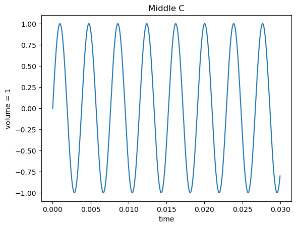
A musical note’s pitch (whether it’s a C, C#, or just plain out-of-tune) is its frequency. For example, middle C (the key in the center of a piano) is a sine wave with a frequency of about 262 Hz (times per second), so it takes that sine wave about .0038 seconds to repeat.

import numpy as np
import matplotlib.pyplot as plt

C_FREQUENCY = 262
time = np.linspace(0, 0.03, 1000, endpoint=False)
sine = np.sin(2 * np.pi * C_FREQUENCY * time)
plt.plot(time, sine)
plt.title('Middle C')
plt.xlabel('time')
plt.ylabel('volume = 1')
plt.show()

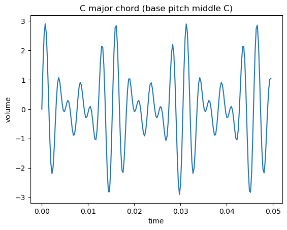
A chord is multiple notes (multiple frequencies) played at the same time. The ratio between the frequencies generally determines how it sounds to your ear: a major chord, which has three frequencies at a $4:5:6$ ratio sounds sweet, and the “panic chord” (which is the two notes of the Jaws theme, played at the same time), which aptly-sounds panic-inducing, has two pitches at a $15:16$ ratio.

I’m giving a “middle school music class” overview of music theory to motivate this. For my fellow nerds I’m assuming just intonation (for simplified ratios) and that we’re whistling (or some other pure sine wave) our notes, not using an actual instrument with overtones. I’m also calling a dyad a chord. My music coursework taught theory with lame ass genres like baroque, classical, and jazz, no Meshuggah or anything else interesting.

A chord is an example of a waveform, which is a sum of sine (or cosine, same thing) functions of different periods. Here’s a C major chord, which is a C, E, and a G (which have the aforementioned $4:5:6$ ratio):

def generate_note_samples(pitch, n_samples=1000, sampling_duration=0.05):
    time = np.linspace(0, sampling_duration, n_samples, endpoint=False)
    pitches = np.sin(2 * np.pi * pitch * time)
    return time, pitches

N_SAMPLES, SAMPLING_DURATION, C_FREQUENCY_HZ, TIME_START_S = 2_048, 0.5, 262, 0
e_frequency, g_frequency = (5/4) * C_FREQUENCY, (6/4) * C_FREQUENCY

c_time, c_pitches = generate_note_samples(C_FREQUENCY, n_samples=N_SAMPLES, sampling_duration=SAMPLING_DURATION)
_, e_pitches = generate_note_samples(e_frequency, n_samples=N_SAMPLES, sampling_duration=SAMPLING_DURATION)
_, g_pitches = generate_note_samples(g_frequency, n_samples=N_SAMPLES, sampling_duration=SAMPLING_DURATION)
c_major_chord = sum([c_pitches, e_pitches, g_pitches]) 

plt.plot(c_time[:N_SAMPLES//10], c_major_chord[:N_SAMPLES//10])
plt.title('C major chord (base pitch middle C)')
plt.xlabel('time')
plt.ylabel('volume')
plt.show()

You can also represent that waveform differently: just show the different frequencies it’s made up of on the x axis. This is generally a more helpful view.

plt.scatter([C_FREQUENCY_HZ, e_frequency, g_frequency], [1, 1, 1])
plt.title('C major chord (base pitch middle C)')
plt.xlabel('frequency')
plt.ylabel('volume')
plt.show()

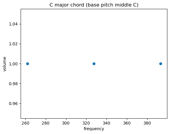
Remember domain and range from middle school pre-algebra, where you learn that a function is a machine on an assembly line that transforms something (from its domain) into something else (from its range), and you plotted the domain of a (univariate…) function on the X axis and the range on the Y? I’ve done the same thing here: the first two plots are a waveform in the time domain, and that last one is in the frequency domain.

What’s the Fast Fourier Transform?

In general, a “Fourier transform” is an algorithm that transforms a waveform in time domain (the first two plots) into its frequency domain (that last plot). The Fast Fourier Transform does that fast ($O(n\;lg(n))$, to be specific).

Bear in mind that computers don’t operate on continuous real numbers: everything’s in binary on those transistors. Those plots of notes and chords look nice and continuous, but they’re actually discrete samples of amplitude at given points in time. The FFT operates on those discrete samples, which is where its other name, the Discrete Fourier Transform, comes from.

How’s the algorithm work?

Using as little math as possible, I’ll provide a naive $O(n^2)$ algorithm (like Bubble Sort) to find a discrete Fourier transform, and then point out some structure in the problem we can exploit to get the FFT, an asymptotically-faster algorithm (like Merge Sort).

Naive Fourier Transform Algorithm

So we have $n$ samples of an an original signal \(X = X[0], X[1], ..., X[n]\) and each $X[i]$ is a real number (an amplitude). The Naive Fourier Transform (NFT) (no, not that one) is to take samples of a sine wave at some frequency \(Y = Y[0], Y[1], ..., Y[n]\) and check how well each sample matches the one. You repeat this for $n$ different possible frequencies $k$ of $Y$, which gives you the $O(n^2)$ time complexity. That yields this “algorithm”:

naive_fourier_transform_outline :: N discrete samples of waveform x (in time domain) -> frequency domain representation of x
    initialize output array X of length N, such that X[i] is how well the wave with frequency i matches x
    
    for each sample n from 0 to N - 1:
        for each frequency k from 0 to N - 1:
            X[k] = how well x[n] matches samples of a wave of frequency k // TODO
    return X

Now, once we have some mathematical formulation of “how well a sample of [our waveform] matches samples of a wave of frequency k,” we have an implementable algorithm.

Sine and Cosine

So, first off, we’re going to be using complex numbers $a + bi$. This is because we’re decomposing a a waveform (some complicated periodic function) into simple periodic functions: sine and cosine waves. A cosine wave is the same wave as a sine wave, though: just shifted horizontally by $90\deg$. Complex numbers allow us to express that “sameness” with Euler’s formula:

\[e^{i\theta} = \cos(\theta) + i\sin(\theta))\]

The cosine is the real part, and the sine is the imaginary part. Still the same wave, defined by $\exp(i\theta)$ (calling $e^x = \exp(x)$ for notational simplicity).

Complex Roots of Unity

Back to frequencies: we’re trying to find the periods of sine and cosine waves (in their complex-numbered formulation, remember) that effectively decompose a signal, which involves guessing-and-checking “how well the given frequency (that we’re testing in our algorithm) fits the samples of the one we’re decomposing.”

The quantity “how well the given frequency (that we’re testing in our algorithm) fits the samples of the one we’re decomposing,” is called a complex root of unity. (It has that name because it’s useful for other things, but that’s what it does for our purposes.)

Derivation: Complex Roots of Unity

I’ll start with what we’re looking for: \(\text{complex root of unity} = \exp(-2\pi i \frac{k}{N} n)\)

We know that how many times a (co)sine wave repeats in a time interval is called its frequency $f_k$. (Like Hz, which is cycles per second.) We’re have $N$ discrete samples of that wave; those are evenly spaced, with $\Delta t$ (a short interval) between them. That gives us a formula for $y[n]$, the value of our (co)sine wave’s amplitude $y$ at sample $n$:

\[y[n] = \text{(co)sine}(2\pi f_k n \Delta t)\]

Now, remember from my previous kernel-related posts that an inner product $\langle x, y \rangle$ measures similarity between two vectors $x$ and $y$. The intuition here is that we’re going to treat $y[n]$ and $x[n]$ (the $n$th sample of the input waveform) as vectors how take their inner product to find their similarity and take:

\[\text{similarity}(y[n], x[n]) = \langle y[n], x[n] \rangle = \langle \text{(co)sine}(2\pi f_k n \Delta t), x[n] \rangle\]

-which gives the similarity between those two samples. If you sum over each $n \in N$, that gives you the similarity a complicated waveform and a simple (co)sine wave, based on their samples.

I’ve been writing (co)sine because, as we know, the sine and cosine at a given frequency are the same wave, just shifted $90\deg$. We can express that “sameness” with Euler’s formula, as I mentioned; we’ll substitute it in where I wrote (co)sine:

\[\begin{align} \text{similarity}(x[n], y[n]) &= \langle y[n], x[n] \rangle \\ &= \langle \cos(2\pi f_k n \Delta t) - i \sin(2\pi f_k n \Delta t), x[n] \rangle \end{align}\]

Then we substitute in $e^{i\theta} = \cos(\theta) + i\sin(\theta))$ to get a simplified expression:

\[\text{similarity}(x[n], y[n]) = \langle \exp(-2\pi i f_k n \Delta t), x[n] \rangle \\\]

In practice, the “inner product” thing was just to notate “similarity.” These two vectors are a complex and a real number (which is a specific type of complex number; all real numbers $a$ are complex numbers $a + 0i$):

\[\text{similarity}(x[n], y[n]) = \exp(-2\pi i f_k n \Delta t) x[n]\]

After substituting in \(f_k = \frac{k}{N \Delta t}\) -we have what we were looking for: how well a sample of a (co)sine wave at a given frequency $f_k$ matches a sample of a complicated, arbitrary waveform. The matching of the waveform and that wave overall is just their sum. That gives the following imperative pseudocode (as well as my declarative, less-slow Python implementation):

naive_fourier_transform :: N discrete samples of waveform x (in time domain) -> frequency domain representation of x
    initialize output array X, such that X[i] is how well the wave with frequency i matches x
    
    for each sample n from 0 to N - 1:
        for each frequency k from 0 to N - 1:
            root_of_unity = exp(-2i * pi * (k / number of samples) * n)) 
            X[k] += x[n] * root_of_unity
    return X

def nft(x):
    N = len(x)
    n = np.arange(N)
    k = n.reshape((N, 1))
    return np.sum(x * np.exp(-2j * np.pi * k * n / N), axis=1)

def fft_to_top_freqs(X, sampling_duration=0.05, top_k=3):
    N = len(X)
    fs = N / sampling_duration # sampling frequency, Hz
    magnitudes = np.abs(X)
    positive_frequencies = magnitudes[:N//2]
    peak_bins = np.argsort(positive_frequencies)[-top_k:][::-1]
    peak_freqs = (peak_bins / N) * fs
    return peak_freqs

X_nft = nft(c_major_chord)
pitches_recovered_by_nft = fft_to_top_freqs(X_nft, SAMPLING_DURATION)
actual_pitches = [C_FREQUENCY, e_frequency, g_frequency]
print(f'actual pitches: {actual_pitches}\npitches recovered by nft: {pitches_recovered_by_nft}') 

actual pitches: [262, 327.5, 393.0]
pitches recovered by nft: [262. 328. 394.]

def plot_frequency_domain(X, sampling_duration):
    N = len(X)
    fs = N / sampling_duration
    magnitudes = np.abs(X)
    positive_frequencies = magnitudes[:N//2]
    normalized_positive_frequencies = 2.0 / N * positive_frequencies
    x_freq = np.linspace(0.0, fs / 2.0, N // 2)
    plt.plot(x_freq, normalized_positive_frequencies)
    plt.title('Pitches of C major recovered by Naive Fourier Transform')
    plt.xlabel('Frequency')
    plt.xlim(0, 500) # so we can see better
    plt.show()

plot_frequency_domain(X_nft, SAMPLING_DURATION)

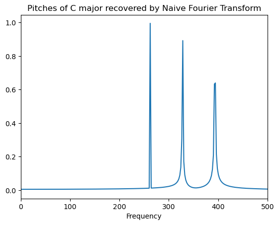
Awesome: we have a correct implementation. Now, let’s optimize the runtime.

A Faster Fourier Transform

I mentioned before that there’s some underlying structure in the “Fourier transform” problem (that our NFT algorithm solves) that allows us to optimize from quadratic to linearithmic time complexity, like from Bubble Sort to Merge Sort.

This “optimize an algorithm by exploiting underlying structure in a problem” thing is generally a theme in LeetCode-style algorithm design: for example, if you’re reusing computation in one of the ubiquitous weakly NP-complete “find optimal subset” problems, you can cache it dynamic programming-style, cutting your time complexity down from exponential to pseudo-polynomial.

The intuition for the hidden structure in the “Fourier transform” problem is that we’re reusing computation: the $n$th and $n+1$th “similarity between sample of some frequency” are related.

The “NFT”

The “NFT” algorithm is just a function that explicitly computes this formula for all possible frequencies $k$:

\[X[k] = \sum_{n=0}^{N-1} x[n] \exp(-2 \pi i \frac{k}{N} n)\]

Now, key insight: if we rephrase that sum by splitting it up into even and odd values of $n$, we get:

\[\begin{align} X[k] &= \sum_{n=0}^{\frac{N}{2} -1} x[2n] \exp(-2 \pi i \frac{k}{N} (2n)) \\ &+\sum_{n=0}^{\frac{N}{2} -1} x[2n + 1] \exp(-2 \pi i \frac{k}{N} (2n + 1)) \end{align}\]

Pay close attention to the similar $(2n)$ and $(2n+1)$ terms: we can factor out the $1$ in there. That gets us, paying close attention to the order of operations:

\[\begin{align} X[k] = &\sum_{n=0}^{\frac{N}{2} -1} x[2n] \exp(-2 \pi i \frac{k}{N} (2n)) \\ + &\sum_{n=0}^{\frac{N}{2} -1} x[2n + 1] \exp(-2 \pi i \frac{k}{N} (2n)) \\ * &\;\exp(-2 \pi \frac{k}{N} (1)) \end{align}\]

Do you see the symmetry? Pay attention to the order of operations there: the second additive term is very similar to the first: scaled, and odd rather than even indices. We just decomposed a DFT into two equally-sized DFTs:

\[\text{DFT}_{total} = \text{DFT}_{even\;indices} + \text{DFT}_{odd\;indices} * \;\exp(-2 \pi \frac{k}{N} (1))\]

That $\exp(-2 \pi \frac{k}{N} (1))$ that relates the odd-indexed and even-indexed DFTs is called a “twiddle factor.” I’m not sure why, either.

That’s enough to implement a divide-and-conquer algorithm to implement that recursive relationship.

def fft(x):
    n = len(x)
    if n <= 1:
        return x
    else:
        fft_evens = fft(x[::2])
        fft_odds = fft(x[1::2])
        twiddle_factors = np.exp(-2j * np.pi * np.arange(n//2) / n)
        res = np.concatenate([fft_evens + twiddle_factors * fft_odds, 
                              fft_evens - twiddle_factors * fft_odds])
        return res

X_fft = fft(c_major_chord)
pitches_recovered_by_fft = fft_to_top_freqs(X_fft, SAMPLING_DURATION)
actual_pitches = [C_FREQUENCY, e_frequency, g_frequency]
print(f'actual pitches: {actual_pitches}\npitches recovered by fft: {pitches_recovered_by_fft}') 

actual pitches: [262, 327.5, 393.0]
pitches recovered by fft: [262. 328. 394.]

Merge Sort, for reference:

def mergesort(x):
    n = len(x)
    def merge(first_half, second_half):
        ...
    if n <= 1:
        return x
    else:
        sorted_first_half = mergesort(x[:n])
        sorted_second_half = mergesort(x[n:])
        return merge(first_half, second_half)

My algorithms hot take is that the FFT and Merge Sort are the same algorithm.

Now, the actual ML: Fourier Transforms of Kernels

That sure was a long digression to introduce an algorithm that can be implemented in less than 10 lines of code.

We’ll be using a library implementation from here on out; you’ll notice that my FFT needs its input to be a power of 2 long, and it’s recursive, which results in probably 37,000 calls to malloc for every single activation record. Gotta love Python.

Anyway, the FFT is a super important algorithm, but doesn’t show up much in machine learning-related things. One use I thought of for it was in stationary-enough univariate time series forecasting, which also has the whole “periodic function” thing and is ML-adjacent data science. But in practice, that’s not an area that I’m super familiar with, and I don’t want to put my foot in my mouth on the internet.

Fourier transforms are useful for many other things besides modeling explicitly periodic functions, though. In general, $e^{ix}$, our sine/cosine waves, form a natural basis for things that are translation-invariant. Images are another “object” whose operators are translation-invariant, so the FFT applies, just from space rather than time: low-frequency components are things that don’t change dramatically from pixel to pixel, like how a picture of the sky doesn’t change much, and high-frequency components are things that do, like how a picture of a building has sharp edges that do have dramatically varying nearby pixels.

One last thing that’s both relevant to machine learning and invariant to translation is many kernels: the things we use to draw expressive nonlinear curves for modeling without spending too much money on cloud GPUs. Look at the radial kernel:

\[\text{radial kernel}(a, b) = \exp(- \lVert a - b \rVert^2)\]

You can see that the values of $a$ and $b$ don’t actually matter; what matters is their difference. You could just as easily write it like:

\[\text{radial kernel}(dist) = \exp(- \lVert dist \rVert^2)\]

The FFT (well, Fourier analysis specifically…) is useful for any kernel (which takes in two objects) that can be expressed as a one-argument function of their difference because those kernels are translation-invariant (and symmetric, and positive semi-definite). There’s a mathematical result called Bochner’s Theorem that says that the Fourier transform (which we just cooked up an algorithm to do) of a (PSD shift-invariant) kernel is a probability distribution. That implies that you can sample from the Fourier transform of some kernel, which is a probability distribution, to approximate it.

The primary motivation for this is scalable kernel-based ML systems: computing a kernel matrix takes $O(n^2)$ time and space, which doesn’t work for Big Data, but if you approximate it with $d$ features, that’s $O(nd)$, and you can make $d = O(1)$ and get an astonishingly accurate approximation, even with small $d$ (like, 1000 dimensions). This is the core idea of Random Fourier Features (sklearn.kernel_approximation.RBFSampler()), which makes you features sampled from the radial/Gaussian kernel’s Fourier transform.

Another reason this is applicable is because attention in a (sequencey, like a LSTM, or Transformer with positional encoding) neural network intuitively computes similarities between sequence elements (dot-product attention to compute that similarity, remember?), so people have used these kernel approximations to design new Transformer-adjacent architectures like the Performer.

If the day job doesn’t work out I might just take my linear algebra straight to Paul Graham and his function fixed-point-finding factory in the Valley, talking some nonsense about “AGI through nonlinear attention” or some word salad like that.

In practice, this evening, we’ll be using this technique to design nonlinear features to “kernelize” a logistic regression, allowing it to draw better decision boundaries than the linear one it ordinarily does.

Random Fourier Features

While Random Fourier Features is one of my favorite ML papers of all time, I’ve made you sit through a ton of math today, so I’ll try and keep it brief. Here’s a link to the paper, which you should definitely read: https://people.eecs.berkeley.edu/~brecht/papers/07.rah.rec.nips.pdf, and https://gregorygundersen.com/blog/2019/12/23/random-fourier-features/ for a more-rigorous explanation.

The idea of Random Fourier Features is a straightforward implementation of that Bochner’s Theorem idea of “you can sample from a kernel’s Fourier transform, which is a probability distribution, to generate features that approximate it.” It goes sort of like:

kernel_sample_transformer :: kernel_function -> X_dataset -> Z_dimension -> Z_dataset
    unnormalized = fourier_transform(kernel_function)
    probability_distribution = unnormalized / k(0, 0)
    // or you could skip this, derive corresponding pdf, and generate the samples in closed form
    // like random normal for the radial kernel

    // each omega in omegas is a vector in input dimension
    omegas = array of (n_features // 2) samples from probability_distribution

    random_projection = omegas @ X
    scaling_factor = sqrt(2/n_features)
    cp = cos(random_projection)
    sp = sin(random_projection)
    Z = hstack(cp, sp)
    Z = Z * scaling_factor
    
    return Z 

// usage
// Z = kernel_sample_transformer(some_kernel_function, X, 1000)
// linear_model(Z, y) will model better than linear_model(X, y) for a nonlinear problem
// It'll also be faster at scale than kernel_model(X, y)

As far as a simple meaning for the sine and cosine here, we know that any function of one input, including the kinds of kernels we can use this with, can be modeled as a sum of sine waves of different frequencies. The kernel is a similarity, so when the difference between its two inputs are smaller, it returns a higher value: where the (co)sine waves add up. Likewise, when the difference between the two inputs is bigger, they’re dissimilar, and the kernel returns a lower value: the sine waves cancel out.

To be completely clear, discretizing a kernel (via finding its result of a grid of inputs) then using the Fast Fourier Transform to approximate its probability distribution, then sampling from that, probably isn’t the best idea, for numerical convergence reasons. In practice, you implement RFFs by analytically finding the kernel’s Fourier transform and sampling from that resulting probability distribution.

So, we’re reimplementing RBFSampler?

Like every clickbait title involving a question, the answer is always no. That’s no fun!

We know that the choice of the model you use on a problem corresponds with a prior belief you have about the nature of its answer.

without descending into Bayesian purist insanity.

We know a logistic regression or a linear SVM draw a hyperplane to separate classes, which corresponds with the prior belief of there being a clean hyperplane in ambient space to split up your data’s classes.

Conversely, Random Forests and XGBoost draw nonlinear, axis-aligned splits to draw nonlinear but “rough” decision boundaries. Lastly, we know that “smooth function approximators” like the radial kernel-equipped SVM and neural networks of all kinds draw smooth, almost analytic-looking decision boundaries. In particular, the simplest radial kernel

\[\text{radial kernel}(a, b) = e^{(- \lVert a - b \rVert^2)}\]

is infinitely-differentiable.

That’s why I wrote it as $e^{\Delta}$ rather than $\exp(\Delta)$!

Just like how nondifferentiable functions aren’t smooth, infinitely-differentiable functions are very smooth. That corresponds with a prior belief that the decision boundary that separates classes is also very smooth. That’s generally not the most optimal one: the reason RF/XGBoost generally works the best on real-world tabular classification problems relative to them (or neural networks)

No Free Lunch still applying; we’re talking about real-world empirical performance here

is probably because the nonlinear-but-rough decision boundaries they draw are better suited to those datasets than the smooth ones neural networks do.

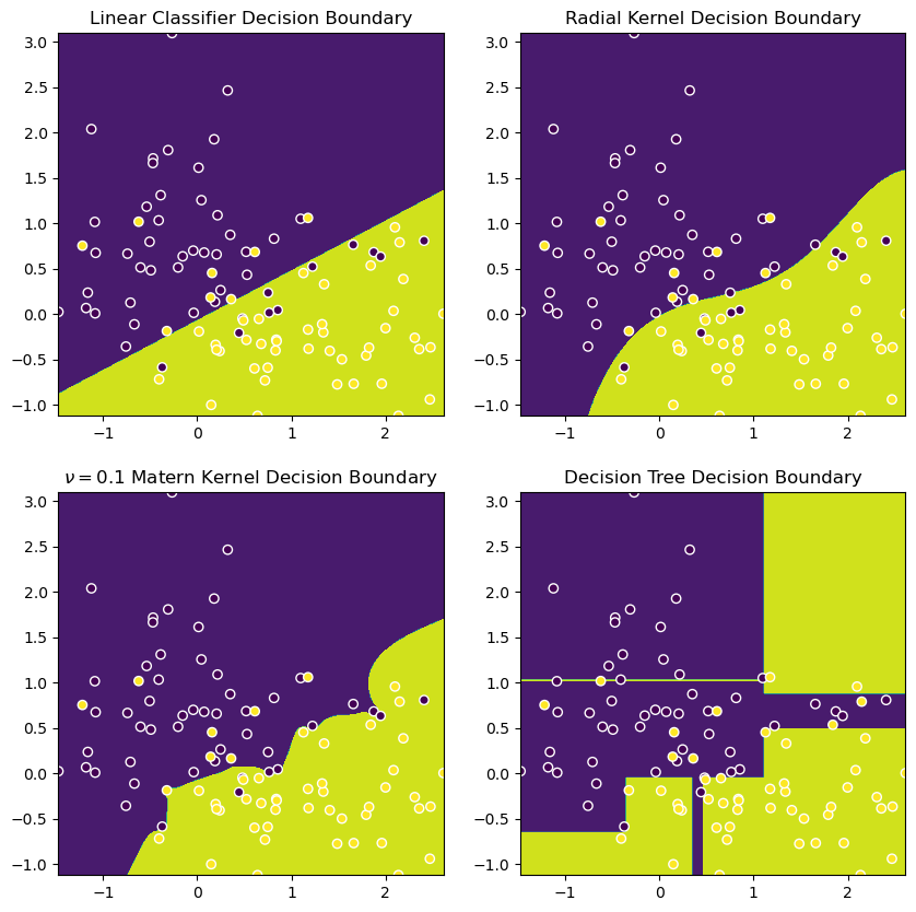
We’re going to be using the FFT to generate samples from a what’s called a Matern kernel, which is a generalization of the radial kernel that allows users to control its “roughness.” The Matern kernel’s roughness is controlled by a parameter $\nu$: lower $\nu$ makes a rougher decision boundary, and higher makes it smoother, with $\nu = \infty$ being the radial kernel.

Besides, sklearn already implements it. Where’s the fun in that?

Here are some visuals to compare their respective decision boundaries, alongside a plain-old logistic regression (which is a linear decision boundary) and a decision tree (XGBoost looks something similar).

import sklearn

X, y = sklearn.datasets.make_moons(random_state=69, noise=0.5)

def decision_boundary(model, model_name, ax, X, y):
    RES = 400
    f1, f2 = np.meshgrid(
        np.linspace(X[:, 0].min(), X[:, 0].max(), RES),
        np.linspace(X[:, 1].min(), X[:, 1].max(), RES)
    )
    grid = np.vstack([f1.ravel(), f2.ravel()]).T
    fitted = model.fit(X, y)
    preds = np.reshape(model.predict(grid), f1.shape)
    display = sklearn.inspection.DecisionBoundaryDisplay(xx0=f1, xx1=f2, response=preds)
    display.plot(ax=ax)
    display.ax_.scatter(X[:, 0], X[:, 1], c=y, edgecolor='white')
    ax.set_title(model_name)

plt.figure(figsize=(10, 10))
decision_boundary(sklearn.linear_model.LogisticRegression(), 'Linear Classifier Decision Boundary', plt.subplot(221), X, y)
decision_boundary(sklearn.svm.SVC(kernel='rbf'), 'Radial Kernel Decision Boundary', plt.subplot(222), X, y)
decision_boundary(sklearn.svm.SVC(kernel=sklearn.gaussian_process.kernels.Matern(nu=0.1)), '$\\nu = 0.1$ Matern Kernel Decision Boundary', plt.subplot(223), X, y)
decision_boundary(sklearn.sklearn.tree.DecisionTreeClassifier(max_depth=5), 'Decision Tree Decision Boundary', plt.subplot(224), X, y)
plt.show()

So, we’ll now do a little experiment to see if we can’t “kernelize” our Logistic Regression with a nice Matern kernel. We’ll:

1. Implement a kernel_sample_transformer, which approximates it with random Fourier features of FFT-found frequencies, and use it with a logistic regression in a pipeline, then
2. Compare the performance of our sampled implementation with that of regular logistic regression.

Now, what we’re going to do is take the FFT of samples of this Matern kernel to make features for our logistic regression. The key difference between our pseudocode and the implementation is that we’re numerically approximating the Fourier transform with a FFT of its samples. I’m using

I’m reimplementing the kernel itself because the sklearn implementation takes two arguments and first finds their Euclidean distance; we want one that takes their difference/distance directly.

import scipy

def matern(dist, nu=0.1, length_scale=1.0):
    scale = np.sqrt(2*nu) * dist / length_scale
    coef = (2**(1-nu)) / scipy.special.gamma(nu)
    return coef * (scale ** nu) * scipy.special.kv(nu, scale)

def kernel_sample_transformer(kernel_function, X, grid_size=8192, z_dim=500):
    '''
    X is univariate array of vals (to be used in predicting y). 
    Univariate just for demoing toy problem; can be applied on features individually
    '''
    # discretize `kernel_function` by evaluating it on a grid
    np.random.seed(69)
    X_range = np.max(X) - np.min(X)
    grid = np.linspace(1e-10, X_range, grid_size)
    kernel_discretized = kernel_function(grid)
    unnormalized_pdf = np.fft.rfft(kernel_discretized)
    pdf = np.abs(unnormalized_pdf)
    pdf /= pdf.sum()

    freqs = np.fft.rfftfreq(grid_size, d=grid[1]-grid[0])
    omegas = np.random.choice(freqs, size=z_dim, p=pdf, replace=True)[None, :]
    X_col = X[:, None] 
    random_projection = X_col * omegas # `X` is (N_samples, 1), `omegas` is (1, Z_dim), this is (N_samples, Z_dim)
    
    cp = np.cos(random_projection)
    sp = np.sin(random_projection)
    scaling_factor = np.sqrt(2 / z_dim)
    Z = np.hstack([cp, sp]) * scaling_factor
    
    return Z 

from sklearn.datasets import make_circles
from sklearn.linear_model import LogisticRegression

X, y = make_circles(n_samples=1000, noise=0.1, random_state=69)
X_train, X_test, y_train, y_test = sklearn.model_selection.train_test_split(X, y, random_state=69)
k = lambda r: matern(r, nu=0.1, length_scale=0.5)
Z_train = np.hstack([kernel_sample_transformer(k, X_train[:, 0], z_dim=100), kernel_sample_transformer(k, X_train[:, 1], z_dim=1000)])
Z_test = np.hstack([kernel_sample_transformer(k, X_test[:, 0], z_dim=100), kernel_sample_transformer(k, X_test[:, 1], z_dim=1000)])
acc_raw = LogisticRegression().fit(X_train, y_train).score(X_test, y_test)
acc_rff = LogisticRegression().fit(Z_train, y_train).score(Z_test, y_test)
print(acc_raw, acc_rff)

0.432 0.844

You can see that the “kernelized” logistic regression was able to fit its nonlinear data much more closely. Thanks for reading!