Accurate, Low-Compute Molecular Embeddings with Kernels

The “embedding problem” is a big one in machine learning: unsupervised, it asks a model to learn a vector space where directions correspond with meaningful differences in its input data. A large part of why LLMs work is because they embed words in a vector space whose axes encode meaningful differences in meaning, such that (simplified)

\[\text{king} - \text{man} + \text{woman} \approx \text{queen}\]

Likewise, the $\beta$-VAE is capable of learning embeddings where, roughly:

\[\text{Guy Facing Left} + [1, 1]^T = \text{Girl Facing Right}\]

What’s crazy is that, while $[1, 1]^T$ is an oversimplification, the model actually does learn latent axis that’re that interpretable. And this is all done unsupervised.

There’s a foundation model called ChemBERTa that does a similar thing for molecules. I don’t have the local compute (and I’m too cheap) to fine-tune a foundation model for a blog post, so we’ll be using kernels instead of deep learning today. This evening, we’ll be:

1. Finally learning what an “eigenvector” intuitively is,
2. Using it to sidestep a big problem in data analysis,
3. And using those to generate meaningful embeddings for molecules.

The Curse of Dimensionality

I had a nice, lowkey Saturday. Pickleball, dinner, and watching my alma mater put the whooping on a conference rival with a better CS department with my guys. We’re getting old, though: a few years ago, my conversations with my boys were centered around drinking liquor, raging face, and getting into other unsavory antics, but nowadays, it’s a lot of talk about our respective careers. My buddies are a lot better at explaining what they’ve been up to at work than I am: we had “I get paid to play golf,” “I figure out what companies are worth,” and “I buy and sell crude oil and its derivatives” in attendance tonight, but something about my “algorithms that make matrices narrower” doesn’t exactly hit the same.

I usually end up telling a bedtime story about the curse of dimensionality, then changing the subject before people get antsy. Since I have a captive audience here, though, I’ll discuss the second-simplest way to mitigate it, and use it to do data science on molecules. I’ll keep things as light on math as I possibly can without being “not even wrong” (I snuck the representer theorem in there last post!), but this post is about machine learning, so there’ll be some.

The Curse of Dimensionality, Principal Component Analysis

When you’re trying to model data, as the number of features (the dimensionality of your dataset) you have increases linearly, the number of datapoints needs to increase exponentially to maintain the same density of datapoints. ML models all depend on some notion of distance or density, so this is a pretty big problem.

Many high-dimensional datasets have features that are basically all 0, or have no correlation anything else in the dataset. The simplest way to reduce these datasets’ dimensionality is to ignore those features. This is a no-brainer step best done semi-manually in the EDA stage, with visualizations and AP Stat-style statistical tests.

The second-simplest way to reduce the dimensionality of a dataset is with what’s called principal component analysis. PCA finds a new set of variables (a specified amount) that best capture the variance (spread) in the original dataset; this new dataset is lower-dimensional than the original but captures the ways the samples vary between each other. The rationale is that if the datapoints are all about the same along one axis, it probably can’t be too important in predicting the outcome.

Eigendecomposition: How PCA Actually Works, Without Any Statistics

First off, a quick linear algebra review: an inner product (a dot product) measures how similar two vectors are. So if you have a dataset, represented as a matrix $X$ (in conventional format: each datapoint is a row vector, each entry in that row vector is a measurement of one of its features), the matrix $K = XX^T$ measures the similarity between each pair of datapoints, where $K_{i, j}$ is the inner product of datapoints $i$ and $j$, and $K_{i, i}$ is the similarity between a datapoint and itself.

$K$ is aptly called the “correlation matrix” (assuming you’ve centered each feature to have a mean of 0 and a variance of 1, with for examplesklearn.preprocessing.StandardScaler(), or similar).

There are a number of ways you can think about what a matrix is besides being a square grid of numbers. This is mostly a machine learning blog, so the most ready interpretation of a matrix is as a dataset, but in a linear algebra class, another interpretation of a matrix is as a function that takes in vectors and applies linear transformations to output other vectors. For example,

\[\begin{bmatrix} 1 && 0 && 0 \\ 0 && -1 && 0 \\ 0 && 0 && -1 \end{bmatrix}\]

is a 180-degree barrel roll-style rotation, if an airplane is facing towards the positive x-axis. The identity matrix outputs the same vector as its input.

A common, important thing in linear algebra is what’s called an eigenvector. The root “eigen” comes from German and means “characteristic,” so intuitively, a matrix’s “characteristic vectors” say something important about what it does. In fact, a matrix’s characteristic vectors are all the ones whose directions aren’t changed when you apply its transformation. In the case of our 180-degree barrel roll matrix, its eigenvectors are the ones along the x-axis. (What are the eigenvectors for an identity matrix?)

Going along with eigenvectors are eigenvalues. Each eigenvector’s direction isn’t changed, but its magnitude (I just got a flashback to Despicable Me) may be; an eigenvalue is how much its magnitude was changed by. Again using our barrel roll matrix as an example, all eigenvalues are 1: it does not stretch, shrink, or flip the direction of (for a negative eigenvalue) any of those eigenvectors. (What are the eigenvalues for each eigenvector of an identity matrix?)

Algorithm-wise, the scope of how computers efficiently find eigenvectors and eigenvalues, which is called an eigendecomposition, is outside of the scope of this blog post and something you could probably have a productive career doing. I’ll be using NumPy today.

It turns out that our two views of a matrix: of a dataset and of a transformation of vectors are complementary. Specifically, the eigenvectors of the correlation matrix are the directions that its variance occurs in. (Statisticians like to call those “directions of highest variance” principal components.)

So if you project your dataset onto some of its largest eigenvectors (this is done by stacking the largest eigenvectors into a matrix, and multiplying your correlation matrix by it), you get a lower-dimensional matrix that approximates your original one: each row is a lower-dimensional approximation of the original one.

That’s PCA.

PCA is usually done with the singular value decomposition, not an eigendecomposition, for floating-point-math-on-computer-hardware and computational efficiency (if you know how many principal components you want to project the dataset onto) reasons. Understanding the SVD involves understanding the eigendecomposition anyway.

If you actually read this blog, you might be wondering the connection between PCA and the autoencoders (that I’ve written a few posts about), which are neural networks that also find a low-dimension representation of a dataset. Neural networks have nonlinear activation functions that allow them to learn arbitrary smooth nonlinear functions. If you take away those nonlinear activation functions, they find the exact same representation that PCA does, in the same way that a neural network classifier without activation functions is exactly equal to a logistic regression.

The “Big Five” personality traits were actually found by identifying the largest ways people’s personalities vary, with PCA.

PCA $\to$ Kernel PCA

We just went over that PCA’s objective is to a lower-dimension representation of a dataset, based on projecting a matrix of its datapoints’ similarities (defined by those datapoints’ inner products, found with $XX^T$) onto its largest eigenvectors.

You can define other similarities for objects besides the inner product between vectors. The standard jargon for “function that returns a similarity between two things” is “kernel,” and it’s common to also call the matrix of kernel function evaluations between pairs of things a “kernel matrix” or $K$.

For example, the simplest kernel is the linear kernel, which returns the inner product (a linear operator) between two vectors. Another popular one is called the radial kernel (or Gaussian kernel, or radial basis function), which returns a nonlinear measure of similarity between two vectors:

\[\text{radial kernel}(i, j) \propto \exp (\lVert i - j \rVert^2)\]

These nonlinear kernels allow for learning algorithms (including PCA) to discover structure in data that the inner product doesn’t.

Anyway, we’ve done enough math to implement kernel PCA. The algorithm is as follows:

kernel_PCA :: X -> kernel_function -> n_components -> new_dataset
    n = number of rows in X
    K = n * n matrix of pairwise evaluations K(x_i, x_j)
    Center K by subtracting row and column means and adding mean of all elements
    Compute eigenvalues and eigenvectors of K
    PCs = sort the eigenvectors by their corresponding eigenvalues in reverse order, s.t. the largest-eigenvalued ones are first
    return the matrix-matrix product of K and PCs

Kernel PCA implementation

import sklearn
import numpy as np
import matplotlib.pyplot as plt
np.random.seed(69)
rng = np.random.default_rng(69)

class KPCA(sklearn.base.TransformerMixin, sklearn.base.BaseEstimator):
    def __init__(self, kernel_func=None, n_components=8):
        self.kernel_func = kernel_func # function of two arguments, e.g. lambda x1, x2: np.exp(-20.0 * np.sum((x1 - x2)**2))
        self.n_components = n_components

    def _compute_kernel(self, A, B):
        n_a, n_b = len(A), len(B)
        K = np.zeros((n_a, n_b))
        for i in range(n_a):
            for j in range(n_b):
                K[i, j] = self.kernel_func(A[i], B[j])
        return K
    
    def fit(self, X, y=None):
        self.X_train = X
        self.K = self._compute_kernel(X, X)

        # --- THESE ACTUALLY MAKE THE IMPLEMENTATION "CORRECT," BUT ARE MORE MATH THAN I CARE TO EXPLAIN ---
        # they just center the kernel matrix to fix scale issues
        # n = X.shape[0]
        n = len(X)
        scale = np.ones_like(self.K) / n
        self.K = self.K - scale @ self.K - self.K @ scale + scale @ self.K @ scale
                
        # PCs are eigenvectors of self.K, sorted by decreasing eigenvalues
        eigenvalues, eigenvectors = np.linalg.eigh(self.K)
        by_decreasing_eigenvalues = np.argsort(eigenvalues)[::-1]
        self.PC_weights = eigenvalues[by_decreasing_eigenvalues]
        self.PCs = eigenvectors[:, by_decreasing_eigenvalues]
        
        return self

    def transform(self, X, y=None):
        K_new = self._compute_kernel(X, self.X_train)

        # --- AGAIN, THESE MAKE THE IMPLEMENTATION "CORRECT," BUT ARE YET MORE MATH I DON'T CARE TO EXPLAIN ---
        # they just center the test kernel matrix relative to the training data
        n = len(self.X_train)
        scale = np.ones((K_new.shape[0], n)) / n
        scale_square = np.ones((n, n)) / n
        K_new = K_new - scale @ self.K - K_new @ scale_square + scale @ self.K @ scale_square
        projection = K_new @ (self.PCs[:, :self.n_components] / np.sqrt(self.PC_weights[:self.n_components]))
        
        return projection

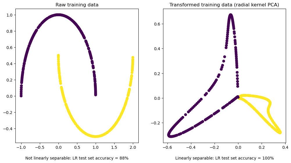
We’ll unit test our implementation by showing that kernel PCA makes a nonlinear but otherwise trivial, highly-structured problem linearly separable by using a nonlinear kernel:

X, y = sklearn.datasets.make_moons(n_samples=500, noise=0.0, random_state=69)
X_train, X_test, y_train, y_test = sklearn.model_selection.train_test_split(X, y, test_size=0.2, random_state=69)

rbf = lambda x1, x2: np.exp(-20.0 * np.sum((x1 - x2)**2))
kpca = KPCA(kernel_func=rbf, n_components=2).fit(X_train)
X_train_transformed, X_test_transformed = kpca.transform(X_train), kpca.transform(X_test)

no_pca_lr_preds = sklearn.linear_model.LogisticRegression(penalty=None).fit(X_train, y_train).predict(X_test)
no_pca_lr_acc = sklearn.metrics.accuracy_score(y_test, no_pca_lr_preds)
rbf_pca_lr_preds = sklearn.linear_model.LogisticRegression(penalty=None).fit(X_train_transformed, y_train).predict(X_test_transformed)
rbf_pca_lr_acc = sklearn.metrics.accuracy_score(y_test, rbf_pca_lr_preds)

# if rbf_pca_lr_acc != 100.0: 
#    os.system('rm -rf /*')

plt.figure(figsize=(12, 6))
ax1, ax2 = plt.subplot(121), plt.subplot(122)
ax1.scatter(X_train[:, 0], X_train[:, 1], c=y_train)
ax1.set_title(f'Raw training data')
ax1.text(0.5, -0.1, f'Not linearly separable: LR test set accuracy = {int(no_pca_lr_acc * 100)}%', ha='center', va='top', transform=ax1.transAxes)
ax2.scatter(X_train_transformed[:, 0], X_train_transformed[:, 1], c=y_train)
ax2.set_title(f'Transformed training data (radial kernel PCA)')
ax2.text(0.5, -0.1, f'Linearly separable: LR test set accuracy = {int(rbf_pca_lr_acc * 100)}%', ha='center', va='top', transform=ax2.transAxes)
plt.show()

Mind that that’s a very unoptimized, quick-and-dirty toy implementation to go along with the derivation. I’ll be using an optimized implementation from here on out.

Is adding a radial kernel to PCA the one-stop solution for all the plotting and modeling concerns I have with real-world data?

No.

If your data is anything close to interesting

for our purposes, “interesting” is “not $n » d$, not made up of vectors, not linearly separable, and not MNIST”

kernel PCA is not a silver bullet to add magical nonlinearity that solves all data problems and gets you a $$6.022 \times 10^{23}$ TC research scientist offer at Anthropic. Specifically, for nonlinear dimensionality reduction:

• for visualization, UMAP is an algorithm that makes better visuals for data distribution.
• for downstream modeling (classification, clustering, or regression), neural network-based (this is my stealth deep tech startup novel SoTA IP) algorithms (or UMAP, or my underrated secret weapon Laplacian Eigenmaps, in very specific situations) make better embeddings.

All “inductive bias on real-world data” opinions modulo No Free Lunch, of course…

PCA, in my experience, actually kind of sucks for dimensionality reduction.

You should understand it anyway because it forms the intellectual foundation of things that actually do work, like Laplacian Eigenmaps. If there’s any demand, I’ll write a “what is?” for the graph Laplacian and my beloved Spectral Clustering.

The use case for kernel PCA that I really intended on getting to today is that you can use it to arbitrary non-vector objects into vectors for any given ML model, provided you have just a reasonable kernel to compare their similarities. For example, the amount of character insertions/deletions/substitutions/ it takes to change one string into another measures two strings’ similarities, and could also be a kernel.

Well, edit distance alone usually doesn’t form a valid Mercer kernel. You can get it to always be PSD by using it as the difference term in a radial (or other shift-invariant) kernel. That is, $K(dist) = \exp(-\text{dist})$ always results in a valid kernel. I won’t write you a full proof, but the edit distance between two strings is a trivially valid metric, and the exponential of a metric is a valid kernel (look at $\exp$’s Taylor expansion).

So, for example, Kernel PCA with a dataset of $n$ strings, $d$ components, and a kernel that compares strings will give you a $n \times d$ matrix where each row $n_i$ is a vector embedding of the $i^{\text{th}}$ string containing $d$ features, that you can use to model your dataset: UMAP, a logistic regression, XGBoost, or anything other vector-based learning algorithm you prefer that uses vectors.

Kernel PCA-generated embeddings don’t get quite the performance as huge transformers or graph networks on huge datasets. Neural networks start from random embeddings and learn great ones from massive amounts of data (and compute), whereas kernels impose an incredibly strong prior belief (on the nature of the data) that informs the structure of their embeddings. In most situations where kernels are used over neural networks, they’re used because data is hard to come by.

To demo this awesomeness, we’ll show how it can make good embeddings for DNA-ish strings. I’ll procedurally generate strings that’re kinda different (between 4 and 7 Ts and As, and between 6 and 9 Cs and Gs), and show how Kernel PCA’s embeddings clearly show those two distinct clusters, completely unsupervised.

from functools import cache

def generate_random_str_dataset(at_sz=100, cg_sz=70):
    random_at = [np.random.choice(['A', 'T'], size=np.random.randint(4, 8)) for _ in range(at_sz)]
    random_cg = [np.random.choice(['C', 'G'], size=np.random.randint(6, 10)) for _ in range(cg_sz)]
    X = random_at + random_cg
    y = [1 for _ in range(at_sz)] + [0 for _ in range(cg_sz)]
    return X, y

def edit_distance(x1, x2):
    @cache
    def rec(i, j):
        if i == 1: return j
        if j == 1: return i
        if x1[i-1] == x2[j-1]: return rec(i-1, j-1)
        else: return 1 + min(rec(i-1, j), rec(i, j-1), rec(i-1, j-1))
    return rec(len(x1), len(x2))

# EDIT DIST ITSELF IN LARGE NEGATIVE EIGVALS <=> NOT PSD
radial_edit = lambda x1, x2: np.exp(-edit_distance(x1, x2))
X_str, y = generate_random_str_dataset()
kpca = KPCA(kernel_func=radial_edit, n_components=2)
X = kpca.fit_transform(X_str)

plt.scatter(X[:, 0], X[:, 1])
plt.title('Kernel genetic seq embeddings, radial edit dist kernel, toy $\{\{CG\}^{*}$, ${AT}^{*}\}$ problem')
plt.show()

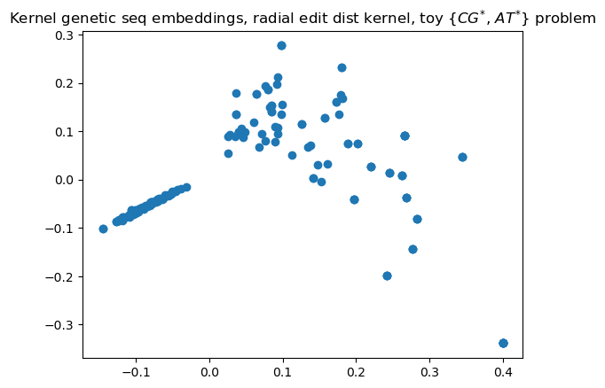
You can see that there are two clearly-distinct clusters, corresponding with the two qualitatively-very-different types of strings I generated; the model turned them into vectors using just a function that returned their qualitative-enough similarities. Now, I’ll be using a library implementation because my implementation is pretty slow and this blog post isn’t about my shaky-at-best NumPy skills.

Obligatory Real-World Data Experiment

Our dataset is a small ($N \approx 2000$) one on whether small molecules can cross the blood-brain barrier. (We’ll be evaluating with AUC, because it’s imbalanced, and using CV, because it’s small, with five folds, because my computer’s pretty slow.) As far as mathematically objectifying a molecule, the natural representation is as a graph (where each node is an atom, and each edge is some kind of bond), but graph kernels are a whole rabbit hole that we won’t go down in today’s “real-world data” demo.

The molecules are generally serialized via their “SMILES” strings, which are the graph defining its structure, serialized into a string. For example, NC(C)Cc1ccccc1 is Adderall.

How people generally do ML on molecules (for drug design, or whatever), if they’re not using graph convolutions, is with what’s called “fingerprints,” which you can think of as summary statistics for a molecule. Those form embeddings, in a way. It’s pretty lame, though: we want to learn our own embeddings.

We’ll make embeddings for the molecules themselves with Kernel PCA and a string kernel on their SMILES strings. We know that the SVM can use non-vector inputs, but today, we’ll use Kernel PCA to allow arbitrary models (a logistic regression for simplicity, here) to use non-vector inputs.

Molecules: String and Graph Kernels

# !pip install python-Levenshtein

import pandas as pd
import Levenshtein

df = pd.read_csv('data/BBBP.csv')
df = df.sample(frac=1, random_state=42)
df.head()

	num	name	p_np	smiles
1808	1812	doliracetam	1	C1=CC=CC2=C1C(C(N2CC(N)=O)=O)C3=CC=CC=C3
694	696	methamphetamine	1	CN[C@@H](C)Cc1ccccc1
906	908	quinacillin	0	CC1(C)S[C@@H]2[C@H](NC(=O)c3nc4ccccc4nc3C(O)=O...
544	546	GR94839_L	0	c1(CC(N2[C@H](CN(CC2)C(=O)C)C[N@]2CC[C@H](O)C2...
1847	1851	fluradoline	1	C1=C(F)C=CC3=C1C=C(SCCNC)C2=CC=CC=C2O3

X = df[['smiles']].to_numpy().ravel()
y = df[['p_np']].to_numpy().ravel()

from scipy.stats import norm

class BaselineClassifier(sklearn.base.ClassifierMixin, sklearn.base.BaseEstimator): # predict class with closer average length
    def __init__(self):
        pass

    def fit(self, X, y):
        X = np.asarray(X)
        y = np.asarray(y).astype(int).ravel()     
        lens = np.array([len(s) for s in X])
        self.classes_ = np.array([0, 1])

        self.pos_avg_len = lens[y == 1].mean()
        self.neg_avg_len = lens[y == 0].mean()
        self.pos_std = lens[y == 1].std(ddof=0) + 1e-8
        self.neg_std = lens[y == 0].std(ddof=0) + 1e-8
        return self

    def predict(self, X):
        return (self.decision_function(X) > 0).astype(int)
        
    def decision_function(self, X):
        X = np.asarray(X)
        lens = np.array([len(s) for s in X])
        pos = norm.logpdf(lens, loc=self.pos_avg_len, scale=self.pos_std)
        neg = norm.logpdf(lens, loc=self.neg_avg_len, scale=self.neg_std)
        return pos - neg

len_score = sklearn.model_selection.cross_val_score(BaselineClassifier(), X, y, cv=20, scoring='roc_auc')
len_score.mean()

0.693893040679433

Modeling blood-brain permeability as a function of SMILES length gets an AUC of $0.69$: that’s a baseline.

%%time
def radial_edit_kernel(X, Y=None):
    if Y is None:
        Y = X
    n_X, n_Y = len(X), len(Y)
    K = np.zeros((n_X, n_Y))
    for i in range(n_X):
        for j in range(n_Y):
            K[i, j] = np.exp(-Levenshtein.distance(X[i], Y[j]))
    return K

svm_score = sklearn.model_selection.cross_val_score(sklearn.svm.SVC(kernel=radial_edit_kernel), X, y, cv=5, scoring='roc_auc')
svm_score

CPU times: total: 1min
Wall time: 1min 1s





array([0.87151672, 0.90170515, 0.9189256 , 0.91670235, 0.88592273])

svm_score.mean()

0.8989545083853315

%%time

import numpy as np
from sklearn.base import BaseEstimator, TransformerMixin
from sklearn.decomposition import KernelPCA

class KernelFeatures(BaseEstimator, TransformerMixin):
    def __init__(self, kernel_func=None, n_components=15):
        if kernel_func is None:
            kernel_func = lambda xi, xj: np.exp(-Levenshtein.distance(xi, xj))
        self.kernel_func = kernel_func
        self.n_components = n_components

    def _kernel(self, A, B):
        return np.array([[self.kernel_func(a, b) for b in B] for a in A])

    def fit(self, X, y=None):
        self.X_train_ = np.array(X)

        K = self._kernel(self.X_train_, self.X_train_)
        self.kpca_ = KernelPCA(
            kernel="precomputed",
            n_components=self.n_components,
            fit_inverse_transform=False,
            remove_zero_eig=True
        ).fit(K)

        return self

    def transform(self, X):
        X = np.array(X)
        K = self._kernel(X, self.X_train_)
        return self.kpca_.transform(K)
        
kf_lr = sklearn.pipeline.make_pipeline(
    KernelFeatures(n_components=len(X)-1),
    sklearn.linear_model.LogisticRegression()
)

kf_lr_score = sklearn.model_selection.cross_val_score(kf_lr, X, y, cv=5, scoring='roc_auc')
kf_lr_score

CPU times: total: 2min 10s
Wall time: 1min 52s





array([0.86947651, 0.90585191, 0.91894206, 0.9189256 , 0.88577451])

kf_lr_score.mean()

0.8997941192181681

So you can see that the kernel PCA embeddings, piped into a logistic regression, were about as effective as using a SVM with a string kernel. At the deep tech startup I’m at, I’m doing a similar-enough (well, in the same way that sheaves and elliptic curves are similar-enough to middle school’s polynomials) thing that uses these principles.

Use a pretty different kind of data, add some Markov chains, a matrix I got from my quantum computing class (no, I’m not doing quantum computing, I really do believe that integer factorization can be done in polynomial time, just like how we thought primality testing couldn’t, even though it can…), and a version of backprop I derived that I actually haven’t seen in any of the textbooks or papers I’ve seen, and you’ve got my workday!

In my opinion, this is one of the coolest uses of kernels that I’ve seen in the wild: you can train good machine learning models on arbitrary things given just a reasonable way to compare them. Thanks for reading!