I feel like my blog posts are getting increasingly “dependency hell”-ish, in that I’m doing an increasingly poor job of making each post’s subject matter’s prerequisite knowledge self-contained in the post, in the name of having a reasonably-interesting narrative. So a “here’s what you missed on Glee” is in order:

Machine learning is commonly done on datasets of vectors (a spreadsheet-like format, $n$ rows $\times$ $d$ columns. Imagine each datapoint as a transaction, with user ID, time spent on our website, number of items purchased…).
There are other kinds of data that could use some machine learning-style insight. A common example is DNA/RNA sequences, which are strings, not vectors.
Certain models can be formulated to use a dataset consisting of inner products (dot products) between the original datapoints (vectors) $X^TX$, rather than the datapoints themselves. Linear (ridge) regression, k-Means clustering, and SVMs are examples of learning algorithms with this property.
An inner product can be thought of as a function that takes in two vectors and returns their similarity.
That means that we can define a function, called a kernel to return a similarity between two non-vector things, like the aforementioned strings.
As long as this kernel is “reasonable” (it’s symmetric and PSD, like an inner product) it actually corresponds with the non-vector datapoints (like DNA sequences) being projected into a (potentially-infinite dimensional) vector (inner product) space, that we can do machine learning in.
Therefore we can cluster strings (or whatever else we can define a kernel on) with k-Means, do regression with ridge regression, or classify with SVMs.
Trivially, PCA can also be expressed in terms of $X^TX$.
Thus, kernel PCA can be used to generate vector embeddings of arbitrary non-vector objects; all you need is a reasonable function to compute their similarity.

We were doing some ML on molecules. When we left off, we cooked up a kernel to compare strings, fit those to a dataset of molecules’ serializations with a simple string kernel, and got a performance metric (competitive with a large foundation model’s after training for a minute or two on an old laptop, as it turns out) data on a benchmark dataset composed of molecules’ string serializations (called SMILES strings).

This was meant to be an illustrative example of a simple kernel between two non-vector things. However, molecules aren’t actually represented as strings. Their structure is two-dimensional (well, three-dimensional, plus rotation over time, so 4D, but 2D is a good representation, so we can use math’s rich study of abstract graphs) not 1D; the SMILES strings do hint to their graph structure, but don’t capture it as well as the actual graph does.

There are kernels between graphs, too. Let’s try one out.

The Weisfeiler-Leman Graph Kernel

What’s a graph?

You intuitively understand what a graph’s mathematical formulation is. Have you seen the Pepe Silvia episode of It’s Always Sunny, where Charlie’s pointing at a complicated web of people, with lines drawn between them to indicate their connections? You can plot relationships between people like that: each person is a node, and each connection (friendship or something else) between those nodes is an edge. Well, a graph’s mathematical formulation is just that: a graph is a collection of nodes, which are things, and edges that connect them somehow. Interpersonal relationships are one thing that you can model with graphs (there’s a billion-dollar idea called Facebook), and websites and the links between them are another (there’s another billion-dollar idea called Google). Molecules can also easily be modeled with graphs: each node is an atom, and each edge is a bond between them. So graph kernels are a useful way to model molecules with machine learning.

Can we make a graph edit distance-based kernel, like our string edit distance-based one?

The string kernel we used on SMILES strings was based on the number of character insertions/deletions/substitutions (the edit distance) between SMILES strings. A SMILES string is a serialization of a molecule’s graph, so it’s something similar to a graph edit distance. However, it’s not exactly equivalent to graph edit distance: in raw SMILES strings, it’s entirely possible that similar molecules have dissimilar serializations.

You can define a kernel based on the graph edit distance to get around that. However, string edit distance is solvable in quadratic time, whereas for arbitrary graphs, it’s a NP-hard optimization problem. There are a variety of schemes to make this slightly more feasible in practice, but in general, this is the wrong tree to bark up.

I tried to think of a good pun, but “a tree is a kind of graph” was the best I could do.

What’s a decent graph kernel, then?

A decent graph kernel is one based on the Weisfeiler-Leman graph isomorphism test (henceforth WLGIT, for brevity).

In the same way that “is this list of numbers sorted” is a problem (that you can solve by checking each element and making sure it isn’t smaller than the one before it), a problem related to graphs is called the “graph isomorphism” problem, which asks, “given these two graphs (collections of nodes and edges between them), can you rename one’s nodes to make it the same as the other one?” (That “you can rename one graph’s nodes to make the other” is “those graphs are isomorphic.”)

The complexity theory community generally thinks that this problem isn’t solvable in worst-case polynomial time, but isn’t NP-complete either: it’s somewhere in between, in a complexity class called “NP-intermediate.” This is the “evidence” behind many people’s gut feeling (myself included) that P $\neq$ NP.

The WLGIT is a heuristic to attempt to solve the graph isomorphism problem. The idea is to rename each node with a new label that contains information about it and its neighbors for a fixed number of iterations $h$. It says whether the two graphs are definitely non-isomorphic after at most $h$ iterations, or if they might be isomorphic, and runs in $O(hm)$, where $m$ is the amount of nodes in the graph.

Remember, though, a kernel is a similarity between two things, and the WLGIT returns a yes/no answer. The WLGIT takes produces $h$ graphs: the $0^{\text{th}}$ is just the node label (of the original graph), the $1^{\text{st}}$ renames the atom to itself and the ones it’s immediately connected to (each atom becomes its neighborhood), the $3^{\text{rd}}$ is a neighborhood of neighborhoods…

If you know graph neural networks, doesn’t this remind you of message passing?

Now, remember that kernels approximate an inner product between its inputs, after some mapping $\phi$ has been applied to them:

\[K(x, y) = \langle \phi(x), \phi(y) \rangle\]

For comparison, for the radial kernel, we implicitly find $\phi$ (which corresponds with an infinite-degree polynomial), but for this kernel, we directly compute $\phi$. For each of those WLGIT-produced graphs of a given graph $x$, $\phi$ is the concatenation of the histogram (a vector of frequencies) of node labels’ frequencies for all of those graphs (numbered from 0 to $h$) that the WLGIT produced:

$\phi_h(x) = |\text{nodes with the first label}|, |\text{nodes with the second label}| ...$ $\phi(x) = [\phi_0(x), \phi_1(x), ... \phi_h(x)]$

And finally, the kernel $K_{WL}(x, y)$ is the sum of each of the WLGIT’s iterations’ histograms’ inner products:

\[K_{WL}(x, y) = \sum_{i=1}^h \langle \phi_h(x), \phi_h(y) \rangle\]

While this isn’t exactly an algorithm analysis blog, this clearly involves a truncated DFS-style thing for $h \in O(1)$ iterations without any kind of subset enumeration, so intuition that this is in polynomial time is accurate. In fact, the label spreading between neighboring nodes’ involves a reasonable ordering which ends up dominating runtimes.

It’s also reasonably useful intuition on “why’s this work?” to note that graph neural networks eventually do just about the same thing: each new feature is a function of an old feature and its neighbors. It turns out that neural networks approach kernel machines as they get bigger and bigger. Maybe material for a future blog post.

Anyway, one of the big benefits of this kernel is that it explicitly computes the feature map (before it returns the explicit, finite-dimensional RKHS inner product $\langle \phi(x), \phi(y) \rangle$). So it doesn’t need to be used with an explicitly kernelized learning algorithm, like the RKHS dual-objective SVM I’m using: if you wanted, you could just use it with a linear SVM, which would allow iterative, $O(n)$-ish minibatch learning with SGD. Basically, this kernel scales.

# !pip install rdkit
# !pip install deepchem

import pandas as pd
import numpy as np
import matplotlib.pyplot as plt
import sklearn
from deepchem.molnet import load_bbbp

import rdkit
import grakel
np.random.seed(69)

tasks, datasets, transformers = load_bbbp(featurizer='Raw')
train_dataset, valid_dataset, test_dataset = datasets
X_train, y_train = train_dataset.ids, train_dataset.y
X_valid, y_valid = valid_dataset.ids, valid_dataset.y
X_test, y_test = test_dataset.ids, test_dataset.y

# fent_row = df.loc[df['name'] == 'fentanyl']
# fent_smiles = fent_row[['smiles']].values[0][0]
fent_smiles = 'CCC(=O)N(C1CCN(CC1)CCC2=CC=CC=C2)C3=CC=CC=C3'
mol = rdkit.Chem.MolFromSmiles(fent_smiles)
img = rdkit.Chem.Draw.MolToImage(mol)
img

png

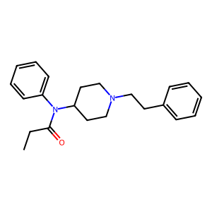
Aromatic Bonds, Avoiding Inbreeding

That’s a fentanyl molecule. One thing you might have noticed is that the WL kernel, as I presented it, assumes every bond (edge) in it is created equal. From high school chemistry, you should remember that not all bonds are the same: you’ve got single, double, and triple bonds, as well as that nice-smelling hexagon-with-three-lines structure on the right and the top left, which has different bonds from all those.

If we were modeling personal relationships, the kernel (as I presented it) would treat a guy who was related to his wife and had a child with his sister the exact same as the expected “child with wife, related to sister.”

This isn’t actually a huge issue on this specific dataset: the difference between benezene and cyclohexane is learned by context clues, implicitly, eventually, and predicting a drug’s blood-brain permeability isn’t really all that contingent on recognizing those. One way to encode that is to encode the outgoing bond types of each atom into its “type,” so instead of the amide’s carbon being a “carbon with three bonds,” we’ll say it’s a “carbon with two single bonds (to the amine and the ethyl) and a double bond (to the oxygen).” For simplicitly, we won’t do that in today’s quick demo, though.

def make_graph(smiles):
    mol = rdkit.Chem.MolFromSmiles(smiles)
    adj = rdkit.Chem.rdmolops.GetAdjacencyMatrix(mol)
    node_labels = {i: atom.GetSymbol() for i, atom in enumerate(mol.GetAtoms())}
    bond_labels = {(bond.GetBeginAtomIdx(), bond.GetEndAtomIdx()) for bond in mol.GetBonds()}
    grakel_graph = grakel.Graph(adj, node_labels, edge_labels=bond_labels)
    return grakel_graph

Sanity Check

%%time

X_train_graphs = np.array([make_graph(x) for x in X_train])
X_valid_graphs = np.array([make_graph(x) for x in X_valid])
X_test_graphs = np.array([make_graph(x) for x in X_test])

wl_h5 = grakel.kernels.WeisfeilerLehman(n_iter=5, normalize=False, base_graph_kernel=grakel.kernels.VertexHistogram)
K_train = wl_h5.fit_transform(X_train_graphs)
K_valid = wl_h5.transform(X_valid_graphs)
K_test = wl_h5.transform(X_test_graphs)

svm = sklearn.svm.SVC(kernel='precomputed', class_weight='balanced', C=0.01).fit(K_train, y_train)
svm_auc = sklearn.metrics.roc_auc_score(y_test, svm.decision_function(K_test))
print(f'SVM with WL kernel AUC: \t{svm_auc}') 

    SVM with WL kernel AUC: 	0.7328258984487908
    CPU times: total: 2 s
    Wall time: 2.03 s

Additionally, this provides competitive performance with deep learning-based approaches: a RoBERTa pretrained on 10 million SMILES strings and fine-tuned for this exact task achieved 0.64 AUC, and a graph neural network achieved 0.71, which are lower than this in an absolute sense. Considering how scalable this is (it’s mathematically equivalent to a linear model with an explicit feature map, which is a combo that plays very nicely with streaming-scale data), I think that’s very impressive.