Scaling Kernel Embeddings, Pt. 1
Quick Review: Vector Embeddings
Remember, we’re talking about sticking arbitrary things into a vector space. To review, kernel PCA is one method:
- Compute a matrix of the things’ similarities. This must be done according to some reasonable function (called a kernel): it must be symmetric and the resulting matrix must be positive semi-definite. The simplest case is a covariance matrix $X^TX$, but the kernel matrix can be thought of as a covariance matrix too.
- Geometrically, the covariance matrix can be thought of as a linear map (it’s still a matrix!) that transforms a spherical dataset into something shaped like a (hyper)football. So its eigenvectors are an orthogonal basis of vectors that describe variance.
- So taking its eigendecomposition and projecting the covariance matrix onto its (largest-eigenvalued) eigenvectors gets you a vector for each datapoint: if you used a string kernel on a dataset of 2000 strings and took the first 20 principal components, you’ll get a 2000x20 matrix, where the 5th row is a 20-dimensional vector embedding of the 5th string.
For more depth check the cute blog post I put out last week.
Kernel PCA $\to$ Diffusion Maps: Intuition
The main prerequisite you’ll need to understand is what a random walk is.
Kernel PCA has some drawbacks. It sticks datapoints into a vector space so as to maximize global variance, which is ultimately a proxy task for “learn underlying structure.” The biggest problem of kernel PCA, though, is that it reflects sampling bias. One of the big assumptions of conventional ML models is iid-ness, which sampling bias clearly violates. Many interesting datasets have train sets’ sampling biased towards higher-density areas and therefore do violate that assumption, though, and today’s diffusion maps help cope with it.
We’re going to make a new mathematically-sound (we already did autoencoders months back, if you’re looking for optimization black magic…) learning algorithm to fix those problems. It’ll take a jump in logic: we’re going to take an abstract similarity matrix (which could still be a kernel matrix, but is commonly found with k-NN) and interpret it as a (weighted or unweighted) graph between datapoints. That is, $A_{i, j}$ is the weight of the edge between node $i$ and $j$ if it exists (or 1 if the graph is unweighted); it’s 0 if the datapoints aren’t similar. From there, we’ll compute the transition matrix of random walks from one node to another (which is $\propto$ the edge weights), which will allow us to compute a different matrix of similarities, called the diffusion matrix, based on how long it takes to go from one point to another after some amount of steps of a random walk. That becomes what we diagonalize.
Just like how dropping food dye into a glass of water results in a visual of dye particles diffusing from where they were dropped throughout the water (this is a mathematically-studied thing), you can think of particles of food dye diffusing between datapoints throughout our similarity graph.
Again: diffusion maps are just like kernel PCA, but we do some funky normalization on $K$ to make the resulting embeddings nicer.
Now, we’ll derive how to implement this all in NumPy.
Diffusion Maps Derivation
For our kernel ridge derivation, I went with the “here’s the intuition (representer theorem), everything is pretty easy from there” route. Today, I think a “start with our hand-wavy intuition, then iteratively add insight until we can basically line-for-line translate to NumPy” route makes more sense, because the actual mathematical justifications for what we’re doing are pretty in-depth and outside of this blog post’s scope. So where we left off is something like:
- Take your similarity matrix $A$. I’m calling it $A$ rather than $K$ because it doesn’t necessarily have to come from a PSD Mercer kernel: it usually comes from k-NN, making it sparse and admitting scalable sparse linear algebra algorithms.
- Form $P$ by dividing each entry of $A$ by its row sum, such that each row’s entries add up to 1. $P$’s rows are now a valid probability density: it’s a Markov transition matrix whose entries are the probability that a random walk starting at one datapoint ends up at the other after one step. (You can then power this matrix by a hyperparameter $t$ to get multiple-step random walks.) ($P$ may no longer be symmetric if we used not-mutual k-NN.) (Rather than manually do it with loops, it makes more sense to define a diagonal matrix $D$ of $A$’s row sums and forming $P = D^{-1}A$.)
- Find $P$’s largest-eigenvalued eigenvectors. That gives you a vector for each datapoint: if you used a string kernel on a dataset of 2000 strings and took the 20 largest-valued eigenvectors, you’ll get a 2000x20 matrix, where the 5th row is a 20-dimensional vector embedding of the 5th string. (2 or 3 could make a nice plot.)
How do we make $P$ symmetric if we used not-mutual k-NN?
If $A$ wasn’t symmetric, we can make $P$ symmetric (while having the same eigenvectors) by instead using $P = D^{-1/2} A D^{-1/2}$.
Okay, so diffusion maps are just a funky normalization of kernel PCA. What about sampling bias mitigation?
That’s one last modification for our algorithm, which’ll introduce another hyperparameter $\alpha \in [0, 1]$. Starting with our original $A$, compute degree (the amount of connected nodes) vectors \(q_{i} = \sum_{j=1}^{n} A_{i,j}\) Then redefine \(A_{i,j} := \frac{A_{i,j}}{q_{i}^{\alpha}q_{j}^{\alpha}}\) The reweighteding to mitigate sampling bias comes from dense sampling regions automatically having larger total edge weights and sparse regions having smaller ones. So a degree vector $q_{i}$ says how “close” $x_{i}$ is to the rest of the dataset. The hyperparameter $\alpha$ is thus “how hard do I want to mitigate sampling density?”
Laplacian eigenmaps, implemented with
sklearn.manifold.SpectralEmbedding, is a special case of this with $\alpha=1$. All this stuff comes from a really neat field of math called spectral graph theory.
That gives a final algorithm:
- Take your similarity matrix $A$, as well as “distance” parameter $t$ (lower $t$ captures local patterns, higher for global geometry) and sampling density corrector $\alpha$.
- Compute degree vectors $q_{i} = \sum_{j=1}^{n} A_{i,j}$.
- Redefine $A_{i,j} := \frac{A_{i,j}}{q_{i}^{\alpha}q_{j}^{\alpha}}$ (to correct for sampling density).
- Compute new degree vectors $d_{i} = \sum_{j=1}^{n} A_{i,j}$, and make a diagonal matrix $D$ out of them.
- Define $P = D^{-1/2} A D^{-1/2}$.
- Find $P$’s largest-eigenvalued eigenvectors.
Let’s implement it. Rather than making it sklearn-compatible (as I usually do), I’ll make it a function, because
unlike, say, an autoencoder, it’s stateless, and embedding “new” datapoints necessarily entails doing the whole thing
from scratch.
import numpy as np
import matplotlib.pyplot as plt
import scipy.spatial.distance as ssd
import sklearn
def diffusion_map(A, t, alpha, k):
    EPS = 1e-12
    q = A.sum(axis=1)
    q = np.power(q + EPS, alpha)

    A = A / (q[:, None] * q[None, :])

    d = A.sum(axis=1)
    D_inv_sqrt = np.diag(1.0 / np.sqrt(d + EPS))

    P = D_inv_sqrt @ A @ D_inv_sqrt

    evals, evecs = np.linalg.eigh(P)
    by_decreasing_evals = np.argsort(evals)[::-1]
    evals = evals[by_decreasing_evals]
    evecs = evecs[:, by_decreasing_evals]

    # largest eigenvector is always eigenvalue 1; discard it
    evals = evals[1:]
    evecs = evecs[:, 1:]

    # take top evecs
    evals = evals[:k]
    evecs = evecs[:, :k]

    # t-length random walks
    evals = evals ** t
    return evecs * evals[None, :]
I didn’t implement the sparse linear algebra, but it’s pretty easy to just drop-in
scipy.sparse.linalgfunctions to approximate (sorta) a kernel with a sparse k-NN graph. This was the idea behind a neat autoencoder thing I did a few months ago. I’m allgergic to the deep learning “who cares about the math lol it works” culture (batchnorm?) but maybe I’ll do some math to justify my machine learning crack smoking and post it one of these days.
Demo: Synthetic Data, Biased Sampling
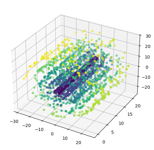
Let’s actually show that when biased sampling density violates iid assumptions, PCA is worse than Diffusion Maps, kernel-for-kernel. We’ll do this by generating biased (inner coils and low height) samples of a swiss roll, which is a super common synthetic dataset for demoing this type of algorithms.
from mpl_toolkits.mplot3d import Axes3D

def biased_roll():
    rng = np.random.RandomState(69)
    inner_frac, height_frac, n, noise = 0.7, 0.7, 3069, 0.25
    t_max = 9 * np.pi
    t = rng.rand(n) * t_max
    h = 21 * rng.rand(n)
    keep_t = rng.rand(n) < (inner_frac * np.exp(-t / t_max) + (1-inner_frac))
    keep_h = rng.rand(n) < (height_frac * np.exp(-h / 21) + (1-height_frac))
    keep = keep_t & keep_h
    t, h = t[keep], h[keep]
    X = np.zeros((len(t), 3))
    X[:, 0] = t * np.cos(t)
    X[:, 1] = h
    X[:, 2] = t * np.sin(t)
    X += noise * rng.randn(*X.shape)
    return X, t

X_roll, y_roll = biased_roll()

fig = plt.figure(figsize=(8,6))
ax = fig.add_subplot(111, projection='3d')
ax.scatter(X_roll[:, 0], X_roll[:, 1], X_roll[:, 2], c=y_roll)
plt.show()
def rbf(X):
    D2 = ssd.squareform(ssd.pdist(X, metric='sqeuclidean'))
    sigma = np.sqrt(0.5 * np.median(D2[D2 > 0]))
    return np.exp(-D2 / (2*sigma**2))

A_roll = rbf(X_roll)
Z_roll_kpca = sklearn.decomposition.KernelPCA(n_components=2, kernel='precomputed').fit_transform(A_roll)
Z_roll_dm = diffusion_map(A_roll, 1, 1.0, 2)
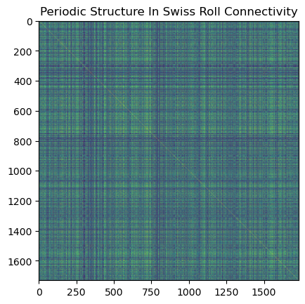
Look at the periodic connectivity patterns in the adjacency matrix: that comes from different arms of the swiss roll being close in ambient space but far along the manifold.
plt.imshow(A_roll, cmap='viridis')
plt.title('Periodic Structure In Swiss Roll Connectivity')
plt.show()
plt.figure(figsize=(10,6))
plt.subplot(121).scatter(Z_roll_kpca[:, 0], Z_roll_kpca[:, 1])
plt.subplot(121).set_title('Kernel PCA Manifold')
plt.subplot(122).scatter(Z_roll_dm[:, 0], Z_roll_dm[:, 1])
plt.subplot(122).set_title('Diffusion Maps Manifold')
plt.show()
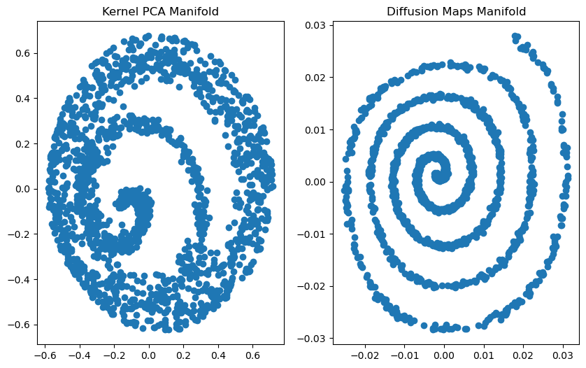
You can see that, with sampling of biased density, PCA failed to unroll the swiss roll: it smushed the outer and inner spirals together. Diffusion maps didn’t, though, despite them using the exact same affinity matrix.
The issue with kernel methods, including Kernel PCA and diffusion maps in their naive formulation (like how I presented the swiss roll), don’t scale: you’ll need a kernel matrix that costs $O(n^2)$ time and $O(n^2)$ space, and a diagonalization, which takes $O(n^3)$ time. That’s fine for smaller datasets (like today’s $n < 40,000$) on modern workstations, but factors like VRAM and PCIe bus bandwidth kill you as data gets bigger and bigger. So when working with kernel methods on bigger datasets, practicioners generally use some approximation of the kernel learning algorithm.
One kernel approximation method that is Random Fourier Features, which I covered in the Fast Fourier Transform entry a few weeks back. It constructs an explicit feature map that approximates the (usually radial) kernel’s implicit one, which you can pipe into some model’s primal form. Concretely, to approximate the almighty RBF SVM, you can use RFFs to make a feature map that you feed into a linear SVM. This is a powerful combo for big data (that is, distributed training-scale data): you can train a linear SVM with streaming SGD, which is how LLMs (that’s definitely big data) are generally trained.
As you can probably tell from my mathematical illiteracy, I have a computer science background, so modeling methods that scale to asymptotically large datasets are intrinsically appealing to me.
A more common (and conceptually much simpler) kernel approximation, though, is conceptually to just throw away a bunch of your training datapoints, keeping $m « n$ of them. This allows us to make a rank-$m$ approximation of the kernel matrix, which we can use for kernel PCA or diffusion maps. While it’s necessary (quadratic time and space complexity is a non-starter for many datasets), it’s actually empirically justified: for many data-kernel pairings, the kernel matrix is low-effective rank: it’s empirically approximated well by a subset of training datapoints.
The sampling from the training data is sometimes done randomly, and it’s also pretty common to run k-means and sample from each cluster. Leverage score-based sampling also works, but defeats today’s purpose of scaling, because it entails a diagonalization of the whole dataset.
An exception I personally found is the Weisfeiler-Lehman kernel on the BBBP dataset, which was our demo in the kernel PCA blog post, which has a pretty flat spectrum: its kernel matrix was pretty close to full-effective rank. That’s why I used
len(X) - 1components. You can check a kernel’s spectrum on some dataset by dividing each eigenvalue by the sum of all eigenvalues, which is interpreted as being the percentage of total variance each corresponding eigenvector’s direction explains.
This blog post isn’t about Nystrom, so just treat it as “low-rank kernel approximation by subsampling that gets slower but more accurate as you increase the number of sampled points, to the limit of the actual $O(n^2)$ kernel.”
import pandas as pd
import numpy as np
import matplotlib.pyplot as plt
import sklearn
from collections import Counter
import scipy.spatial.distance as ssd

import deepchem as dc
from deepchem.molnet import load_hiv
import rdkit
from rdkit import Chem
from rdkit.Chem import AllChem, MACCSkeys, Descriptors, DataStructs
Demo: Real-World Molecules
From last time, we know that diffusion maps and kernel PCA are both diagonalizations of some abstract similarity matrix: kernel PCA is eigendecomposition of a PSD kernel/covariance matrix, and at our level of abstraction, diffusion maps is similar, but with some funky normalization that makes it robust to biased (not proportionate to data density) sampling, as our demo showed. Now, we’re going to run an experiment to see if diffusion maps scale better than kernel PCA: we’ll see if they produce better (as measured by downstream classification) embeddings on the same Nystrom-approximated kernel matrix.
We’ll be using the same MoleculeNet database as last time, but we’ll be using a different dataset today, called “HIV,” consisting of SMILES strings of some 41,000 drugs and their ability to inhibit HIV replication. Like the previous few posts, this also fits the “drugs” theme and should be financially and socially well-motivated enough to count as an interesting real-world problem.
However, unlike the previous few posts, this isn’t about specific (graph) kernels, so we’ll be “vectorizing” molecules in the industry-standard way with what’s called their Morgan, or ECFP4, fingerprints. A molecule’s ECFP4 fingerprint is found by, for all atoms, taking all the other atoms within a given radius (to form a sub-molecule) and converting them into a a set of substructures, which is hashed to form a (usually 2048-long) bitfield. So a Morgan fingerprint is a set, represented as a bitfield. We’ll be using the Tanimoto kernel, which compares two sets similarities’ by the ratio between their intersection and unions’ cardinalities: standard, and super fast with SIMD AND/OR ops.
A Morgan fingerprint is actually found in a reasonably similar way to the Weisfeiler-Lehman graph kernel’s explicit feature map. The Morgan algorithm is actually older than the graph isomorphism heuristic that Weisfeiler and Lehman came up with that forms the idea behind the related kernel. You can use Morgan fingerprints as a feature map for supervised learning too, of course.
So today’s demo is:
- We have our HIV dataset, which is univariate binary classification: $X$ is a molecule’s SMILES string, and $y$ is whether it’s a useful drug (for inhibiting HIV replication).
- Feature engineer $X \mapsto \text{ECFP}(X) \in {0,1}^{2048}$ with RDKit, which is a nice open-source cheminformatics library.
- Nystrom-subsample the dataset. (Uniformly for today. K-means maybe another time.)
- Compute that training-subsampled Tanimoto kernel matrix, for subsampled training datapoints and the test set.
- Use that for kernel PCA.
- Use that for diffusion maps.
- Pipe those into the same classifier and compare performances.
Get our dataset
tasks, datasets, transformers = load_hiv(featurizer='Raw')
train, valid, test = datasets
X_train, y_train = train.ids, train.y
X_valid, y_valid = valid.ids, valid.y
X_test, y_test = test.ids, test.y

print(X_train.shape, y_train.shape)
print(X_test.shape, y_test.shape)
(32896,) (32896, 1)
(4112,) (4112, 1)
Convert X to ECFP fingerprints
%%time

mfpgen = Chem.rdFingerprintGenerator.GetMorganGenerator(radius=2, fpSize=2048)
def SMILES_to_ecfp4(SMILES):
    mol = Chem.MolFromSmiles(SMILES)
    return mfpgen.GetFingerprint(mol)

X_train_ecfp4 = []
for idx, SMILES in enumerate(X_train):
    ecfp4 = SMILES_to_ecfp4(SMILES)
    X_train_ecfp4.append(ecfp4)
    if idx % 2000 == 0:
        print(f'featurized {idx}/{len(X_train)} ({int(idx/len(X_train) * 100)}%)')
print('Done featurizing X_train.')

X_test_ecfp4 = []
for idx, SMILES in enumerate(X_test):
    X_test_ecfp4.append(SMILES_to_ecfp4(SMILES))
    if idx % 2000 == 0:
        print(f'featurized {idx}/{len(X_train)} ({int(idx/len(X_test) * 100)}%)')
print('Done featurizing X_test.')
featurized 0/32896 (0%)
featurized 2000/32896 (6%)
featurized 4000/32896 (12%)
featurized 6000/32896 (18%)
featurized 8000/32896 (24%)
featurized 10000/32896 (30%)
featurized 12000/32896 (36%)
featurized 14000/32896 (42%)
featurized 16000/32896 (48%)
featurized 18000/32896 (54%)
featurized 20000/32896 (60%)
featurized 22000/32896 (66%)
featurized 24000/32896 (72%)
featurized 26000/32896 (79%)
featurized 28000/32896 (85%)
featurized 30000/32896 (91%)
featurized 32000/32896 (97%)
Done featurizing X_train.
featurized 0/32896 (0%)
featurized 2000/32896 (48%)
featurized 4000/32896 (97%)
Done featurizing X_test.
CPU times: total: 11.9 s
Wall time: 12 s
Approximate embeddings
def build_kernel(A, B):
    n_a, n_b = len(A), len(B)
    total = n_a * n_b

    K = np.zeros((n_a, n_b))
    for i in range(n_a):
    #     for j in range(n_b):
    #         K[i, j] = kernel_func(A[i], B[j])
        row = DataStructs.BulkTanimotoSimilarity(A[i], B)
        K[i, :] = np.fromiter(row, dtype=np.float64, count=n_b)
    return K

def nystrom(X, m):
    def invsqrt(W):
        eigvals, eigvecs = np.linalg.eigh(W)
        eps = 1e-9
        inv_sqrt = np.diag(1 / np.sqrt(eigvals + eps))
        return eigvecs @ inv_sqrt @ eigvecs.T

    np.random.seed(69)
    idxs = np.random.choice(len(X), size=m, replace=False)
    # sample = X[idxs]
    sample = [X[i] for i in idxs]
    C = build_kernel(X, sample)
    W = build_kernel(sample, sample)
    Phi = C @ invsqrt(W)
    return Phi

m = 2000 # |X| ~~ 37,000, m=1000 is 16s, m=1500 is 27s
X = X_train_ecfp4 + X_test_ecfp4
Phi = nystrom(X, m)
def kpca_nystrom_embed(Phi, n_components):
    Phi -= Phi.mean(axis=0, keepdims=True)
    K_approx = Phi.T @ Phi
    eigvals, eigvecs = np.linalg.eigh(K_approx)
    decreasing_eigenvalues = np.argsort(eigvals)[::-1]
    eigvals, eigvecs = eigvals[decreasing_eigenvalues], eigvecs[:, decreasing_eigenvalues]
    # Z = Phi @ eigvecs[:, :n_components] / np.sqrt(eigvals[:n_components]) <-- GUARD SMALL EIGVALS
    eps = 1e-12
    inv_sqrt = 1.0 / np.sqrt(np.maximum(eigvals[:n_components], eps))
    Z = Phi @ (eigvecs[:, :n_components] * inv_sqrt[None, :])
    return Z

kpca_embeddings = kpca_nystrom_embed(Phi, m)
def dm_nystrom_embed(Phi, m, d, t):
    d_vec = Phi @ (Phi.T @ np.ones((len(Phi))))
    eps = 1e-9
    D_invsqrt = 1.0 / np.sqrt(d_vec + eps)
    Phi_normalized = D_invsqrt[:, None] * Phi
    K_approx = Phi_normalized.T @ Phi_normalized
    eigvals, eigvecs = np.linalg.eigh(K_approx)
    decreasing_eigenvalues = np.argsort(eigvals)[::-1]
    eigvals, eigvecs = eigvals[decreasing_eigenvalues], eigvecs[:, decreasing_eigenvalues]
    Z = Phi_normalized @ eigvecs[:, :d]
    Z *= (eigvals[:d] ** t)
    return Z

dm_embeddings = dm_nystrom_embed(Phi, m, m, 1)
kpca_embeddings.shape, dm_embeddings.shape
((37008, 2000), (37008, 2000))
Truncate to $\mathbb{R}^{n \times 1337}$
n_dims = 1337
kpca_embeddings_truncated = kpca_embeddings[:, :n_dims]
dm_embeddings_truncated = dm_embeddings[:, :n_dims]

kpca_embeddings_train = kpca_embeddings_truncated[:len(X_train)]
kpca_embeddings_test = kpca_embeddings_truncated[len(X_train):]
dm_embeddings_train = dm_embeddings_truncated[:len(X_train)]
dm_embeddings_test = dm_embeddings_truncated[len(X_train):]

kpca_decision = sklearn.linear_model.LogisticRegression(class_weight='balanced').fit(kpca_embeddings_train, y_train).decision_function(kpca_embeddings_test)
dm_decision = sklearn.linear_model.LogisticRegression(class_weight='balanced').fit(dm_embeddings_train, y_train).decision_function(dm_embeddings_test)
kpca_auc = sklearn.metrics.roc_auc_score(y_test, kpca_decision)
dm_auc = sklearn.metrics.roc_auc_score(y_test, dm_decision)

print(f'kpca embeddings got {kpca_auc}; dm embeddings got {dm_auc}')
kpca embeddings got 0.7330120156087007; dm embeddings got 0.7420333809836572
I’m no statistician, but that seems right to me. Thanks for reading!